Potential outcomes, ATEs, and CATEs

Theory

According to the theory explained in chapter 2 of Mastering ’Metrics, attending a private university should be causally linked to earnings and income—that is, going to a private school should make you earn more money. The type of education you receive, however, is not the only factor that influences earnings. People self-select into different types of universities and choose where to apply and which offers to accept. They also choose to not apply to some schools and are also rejected from other schools. Unmeasured characteristics help determine both acceptance to schools and earnings.

We can draw a simplified version of this causal story with a directed acyclic graph (DAG) or causal model:

dag <- dagify(Y ~ P + G,
              P ~ G,
              exposure = "P",
              outcome = "Y",
              labels = c(Y = "Earnings", P = "Private university", 
                         G = "Student characteristics (group)"),
              coords = list(x = c(Y = 3, P = 1, G = 2),
                            y = c(Y = 1, P = 1, G = 2)))

ggdag_status(dag, use_labels = "label") + 
  guides(color = FALSE) +  # Remove legend
  theme_dag()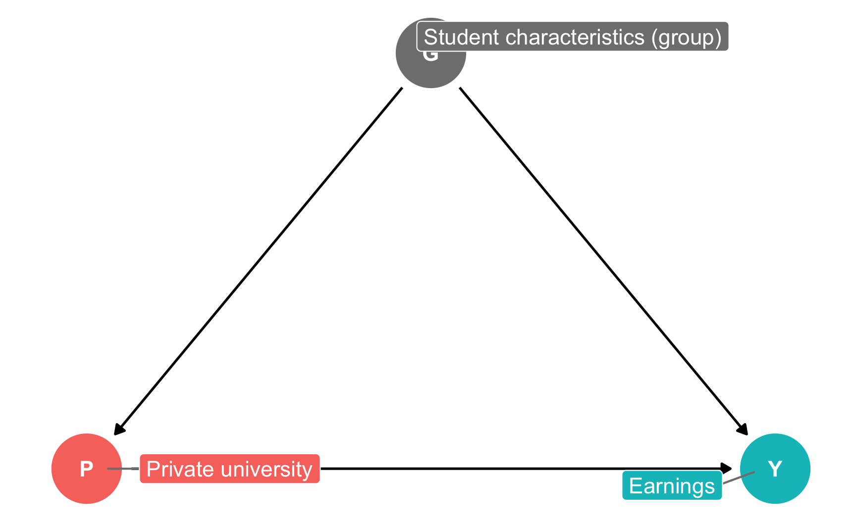

Effect of private school on earnings, no controls

Because we don’t have a time machine, we can’t look at individual-level counterfactuals—we can’t send Person 1 to a private school, watch them for 40 years after, and then go back and send Person 1 to a public school and watch them for 40 years. To get around this, we can instead calculated the average treatment effect, or ATE, and find the average of all individual-level causal effects. We can use the information from our theory’s DAG to calculate a (hopefully!) accurate ATE.

First we load the data from this CSV file (typed from the table in Mastering ’Metrics):

• public_private_earnings.csv

# The data doesn't come with an indicator variable marking if students went to a
# private school, so we create one here. If the string "ivy" is found in the
# enrolled column, mark it as true, otherwise mark it as false.
# 
# We also create a variable that indicates if someone is in group A or not that
# we'll use in the regression models. We could technically just include the
# group variable in the model, where it would be treated as a dummy variable,
# but the reference category would be A, not B, so this is a little trick to
# force it to show results for group A.
schools <- read_csv("data/public_private_earnings.csv") %>% 
  mutate(private = ifelse(str_detect(enrolled, "ivy"), TRUE, FALSE)) %>% 
  mutate(group_A = ifelse(group == "A", TRUE, FALSE))

# Only look at groups A and B, since C and D don't have people in both public
# and private schools. | means "or"
schools_small <- schools %>% 
  filter(group == "A" | group == "B")

It’s really tempting to just find the average income for private school and subtract it from public school, like so:

schools_small %>% 
  group_by(private) %>% 
  summarize(avg_earnings = mean(earnings))

## # A tibble: 2 x 2
##   private avg_earnings
##   <lgl>          <dbl>
## 1 FALSE          70000
## 2 TRUE           90000

It looks like those who went to private school have $20,000 more in earnings! That’s a ton! It’s also incredibly wrong. Don’t do this! This does not account for any confounding or selection bias. According to our DAG, student characteristics are a huge confounder. We need to account for those.

Following the potential outcomes framework, we can find the ATE by combining the conditional ATEs (or CATEs) for subgroups that are likely to predict outcomes or that bunch up similar observations. Let’s use the Group A and B distinction as our subgroups here.

First we can look at the average income for people in each group, divided by whether they went to a private or public school:

avg_earnings <- schools_small %>% 
  group_by(group, private) %>% 
  summarize(avg_earnings = mean(earnings))

avg_earnings

## # A tibble: 4 x 3
## # Groups:   group [2]
##   group private avg_earnings
##   <chr> <lgl>          <dbl>
## 1 A     FALSE         110000
## 2 A     TRUE          105000
## 3 B     FALSE          30000
## 4 B     TRUE           60000

Here we see that group A has higher income on average than group B, regardless of whether they went to a private school. Everyone in group A earns roughly $100,000, while those in group B earn a lot less.

We can find the exact differences in earnings for public vs. private within each group by pulling the values out of the table and taking their differences

# Pulling out each of the numbers is tedious and a good example of why we use
# regression instead. filter() selects rows that match the specified conditions
# (here where group and private both equal something) and pull extracts a column
# from the dataset. Because we're filtering this data in a way that makes it
# only have one row, pull() will extract a single number.

# Group A
income_private_A <- avg_earnings %>% 
  filter(group == "A" & private == TRUE) %>% 
  pull(avg_earnings)

income_public_A <- avg_earnings %>% 
  filter(group == "A" & private == FALSE) %>% 
  pull(avg_earnings)

cate_a <- income_private_A - income_public_A
cate_a

## [1] -5000

# Group B
income_private_B <- avg_earnings %>% 
  filter(group == "B" & private == TRUE) %>% 
  pull(avg_earnings)

income_public_B <- avg_earnings %>% 
  filter(group == "B" & private == FALSE) %>% 
  pull(avg_earnings)

cate_b <- income_private_B - income_public_B
cate_b

## [1] 30000

The private-public earnings gap for people in Group A (or \(\text{CATE}_\text{Group A}\)) is -$5,000, while for Group B (or \(\text{CATE}_\text{Group B}\)) it is $30,000. It seems that there’s a big effect for Group B, but a small reversed effect for A.

We want to account for how many people are in each group, though, since A has more people than B, so we calculate the proportion of each group in the same and multiply the group differences by those proportions.

\[ \text{ATE} = \pi_\text{Group A} \text{CATE}_\text{Group A} + \pi_\text{Group B} \text{CATE}_\text{Group B} \]

# We need to find the proportion of people in each group
prop_in_groups <- schools_small %>% 
  group_by(group) %>% 
  summarize(n = n()) %>% 
  mutate(prop = n / nrow(schools_small))
prop_in_groups

## # A tibble: 2 x 3
##   group     n  prop
##   <chr> <int> <dbl>
## 1 A         3   0.6
## 2 B         2   0.4

prop_A <- prop_in_groups %>% filter(group == "A") %>% pull(prop)
prop_B <- prop_in_groups %>% filter(group == "B") %>% pull(prop)

# With those proportions, we can weight the differences in groups correctly
weighted_effect <- (cate_a * prop_A) + (cate_b * prop_B)
weighted_effect

## [1] 9000

From this it looks like attending a private university causes a bump in earnings of $9,000. This is the average treatment effect (ATE).

Effect of private school on earnings, with regression and controls

Instead of looking at weighted averages (since that’s tedious with just two groups—imagine doing all that with 3+ groups!), we can use a regression model that accounts for differences between groups A and B, since something about group A made them way wealthier than group B regardless of school type.

We do that by predicting earnings based on private/public school attendance while also controlling for group:

model_earnings <- lm(earnings ~ private + group_A, data = schools_small)

tidy(model_earnings)

## # A tibble: 3 x 5
##   term        estimate std.error statistic p.value
##   <chr>          <dbl>     <dbl>     <dbl>   <dbl>
## 1 (Intercept)   40000.    11952.     3.35   0.0789
## 2 privateTRUE   10000.    13093.     0.764  0.525 
## 3 group_ATRUE   60000.    13093.     4.58   0.0445

There are three important numbers here. The intercept (or \(\alpha\) in Mastering ’Metrics, or \(\beta_0\)) is $40,000. This represents the earnings for someone with all the switches and sliders in the model set to 0 or turned off—in this case, someone who went to a public school in group B.

The group_A coefficient shows the effect of just being in that group. For whatever reason, Group A earns an average of $60,000 more than Group B—for reasons other than education. This allows us to control for the effect of selection.

The coefficient for private is the one we care about the most—this is the causal effect of private schools on earnings (assuming we can justify all the controls and the matching into groups). It is $10,000, which means that attending a private school gives you that much of a bump in income. This is larger than the $9,000 we found earlier, but is probably more accurate since we’re accounting for other weighted differences between groups.